 abc
abc
Level I STEP 4 (Linked page)
Repeated measure ANOVA's |
So far we have considered situations where a single value is recorded for each variable within the n factors under investigation. Many experiments and surveys however, need to take readings over a period of time. For example, changes in temperature, changes in weight, pH or height etc. So the repeated measures may be in time or space or they may be taken on individual sampling units after a series of manipulations. Many laboratory drug testing regimes follow this latter pattern as do Ecological / Biological surveys in the natural world..
So now the
two-way ANOVA is going to 'expand' to ascertain whether there is a difference
between treatments
as well as looking for
the variability between individual cases.
As a general point, note how rapidly our data sets can 'grow' seemingly out of control once we start to introduce more variables into the arena. This is an issue that we will be dealing with more fully in STEP 7
 The
Environment Agency monitor the sewage outfall entering rivers in many ways.
One is to take samples from the river beds and identify all the invertebrate
species present. This method gives a quick and simple 'snapshot' of the river
and the presence or absence of certain 'indicator species' can give experts
a clearer picture of the 'health' of that river. The technique also allows
comparative assessment of the biodiversity of these rivers to be made.
Such surveys are usually ongoing and the same sampling locations should always used.
Q. Why do you think this last point is important?
The technique is also of use during an emergency....
There has recently been some considerable flooding in the Dorset / Devon region and river pollution from untreated sewage would constitute a serious health hazard. The agency decided to monitor 5 particular rivers (cases) considered to be at risk.
Four replicated locations on each river were selected: immediately above the sewage outfall, immediately below the outfall, 0.33km downstream and finally, 1km downstream. Note that we are not trying to discern differences between individual rivers.
2 samples were taken (two days after the flooding occurred and one week later) at each location thus giving us a total of: 5 rivers x 4 locations x 2 dates = 40 samples to analyse.
The reason that this has to be a repeated measure test is that a reading was taken at each location twice and separated only by time (1 week). If we had only taken one reading at each location, we would have had only 20 samples to analyse and the Two-factor Independent ANOVA (STEP 4) would have been applicable.
Never forget that we must always begin with (in this case: 3) Null Hypotheses and their Alternatives.
Task: Write them out.
Now here are the results:

Each value represents the total number of species of invertebrate captured within that sample.
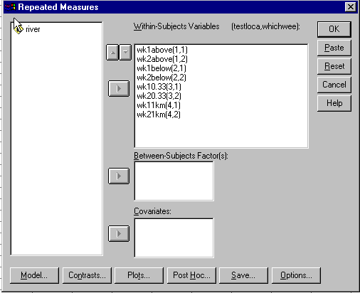
Set up the Variable Table as above, note that we are working with 8 x 5 sets of data. Each of these columns must be entered in 'variable view' as as separate variable, e.g. 'wk1above', 'wk1below' etc. The two factors in the test are 'Test location' (there are 4) and 'Which week' (there are 2).
Go to: Analyse, GLM, Repeated Measures and fill in the window as shown below....
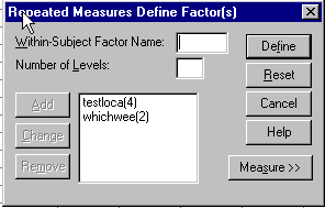
Click Define, the Repeated Measures window appears. Great care must be taken to transfer the correct variable name and place it in the right chronological slot. The window should look like this when completed...
Request a Profile plot in the usual way with 'testlocation' on the horizontal axis and place 'Which Week' in the Separate Lines box. Open Options and tick 'Compare main effects' and 'Bonferroni' and also tick for descriptive statistics. Click OK.
You will note that there is a very large output, much of which can be discarded.
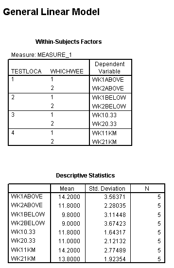
The mean values (of all 5 rivers) of the number of species present are given for all 4 locations (and both weeks) in the table above and shown in the profile chart below. Study this 'profile plot' before moving on.
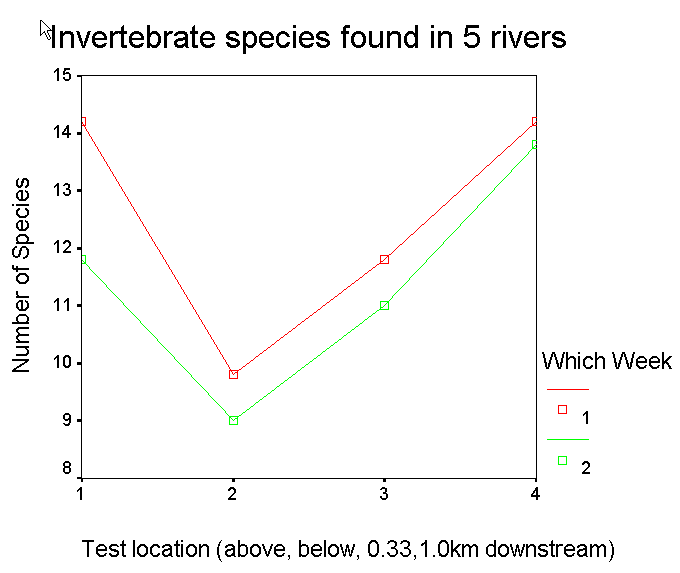
Q. What preliminary deductions can you make? Why might the species count above the outfalls also show a reduction in Wk 2?
Q. Are the downstream results simply a reflection of sewage dilution or is there any evidence of genuine recovery?
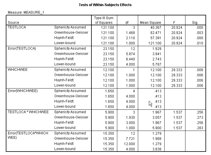
The above table looks daunting but need not be:
Firstly only use the 'Sphericity assumed' rows of data.
|
1) The factor TESTLOCA has a P-value of .000 or less and is therefore significant at the 1% level. Accept H1.1
2) The factor WHICHWEEK has a P-value of .006 and is therefore also significant at the 1% level. Accept H1.2
3) The test for interaction yields a P-value greater than 0.05 (.256) and is therefore NOT SIGNIFICANT i.e. there is no interaction. Accept H0.3 |
We can use mathematical notation to summarise these findings:
TESTLOCA: F( 3, 12) = 20.924; p<0.01
WHICHWEEK: F(1, 4) = 29.333; p<0.01
TESTLOCA*WHICHWEEK: F(3, 12) = 1.537; NS
We can conclude that both factors (Location and Which Week) exhibit 'main effects' and thus have a highly significant bearing upon the numbers of species recorded but that there is no interaction between these two factors. This latter point is borne out by the profile chart.
Q. How and Why?