abc
Level I STEP 6
Other aspects of Multivariate analysis |
As the name implies, this very large topic includes some of the many techniques (MANOVA, PCA, Cluster etc.) that have been developed to cope with numerous variables simultaneously. That is, more than two variables simultaneously. These tests are extensions of bivariate methods already discussed.
By now it will be apparent that the data sets are going to become very large and cumbersome. There are just too many possible investigations that could be made but some will inevitably be more meaningful than others. Our methods need to now extend beyond comparisons of perhaps A, B and C. We are interested in the relationships between many individuals but how to express this is difficult.
Let us suppose that we wish to categorise 100 people. The first and most obvious characteristic to start with is 'male / female'. Next we might consider height (short / tall). Note also that we have only given two choices, the situation becomes even more unwieldy if we had three or more.
So far we only have four possible categories:
Male / Tall (MT)
Male / Short (MS)
Female / Tall (FT)
Female / Short (FS)
If we add a third variable such as eye colour (blue / brown)(bl/br), we now have 8 categories. If we add a fourth, say hair colour (dark / fair)(d/f) (still only two options though) we have 16.
The results might look like this:
|
MTbld |
MTblf |
MTbrd |
MTbrf |
MSbld |
MSblf |
MSbrd |
MSbrf |
|
|
numbers |
6 |
7 |
5 |
8 |
9 |
7 |
7 |
3 |
|
FTbld |
FTblf |
FTbrd |
FTbrf |
FSbld |
FSblf |
FSbrd |
FSbrf |
|
|
numbers |
4 |
6 |
7 |
5 |
6 |
8 |
5 |
7 |
= 100.
To convey all this information in a flat, 2-dimensional way would be difficult. However,if we think of each group as a 'cloud' of individuals floating in a 3-dimensional space a number of possibilities open up. Try and use the idea of an X, Y and Z axis wire plot as the frame for these 'clouds' to sit in. You may think of this as a scattergraph but in 3D. As we have chosen to use 4 variables, we are going to have to think of ways of 'distilling the information' contained in those four variables down to a maximum of three new variables because we only have three axes to usu., Y and Z. This important concept is known as 'data reduction'. It should also be borne in mind that although we have started by considering Ordinal data, it is perfectly feasible to extend the procedure to use Interval and Ratio data as well.
Let us further consider the nature of these 'clouds'. For instance the 'male clouds' are going to overlap with each other because of the 'maleness' and the size of each cloud might convey the proportional numbers (size of category) present. As each component (such as hair colour) is incorporated in the cloud it will slightly change the shape. So we are trying to build up a mental picture of 16 'clouds', all different sizes and shapes but each one representing one of the groups identified above. At this stage, simply try to hold on to this concept.
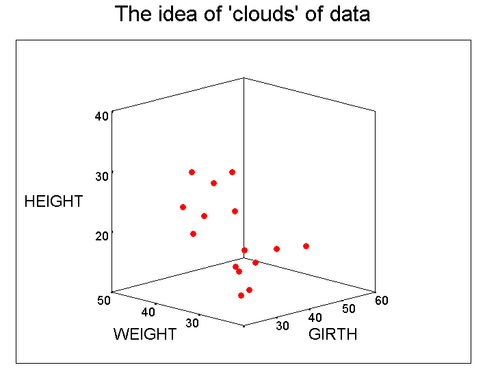
Let us imagine that we have been given the heights, weights and girths of 15 individuals but we have not been told whether they are male of female! If we plotted those three variables on a 3D graph, we produce the following chart...

You should be able to see that there appear to be two 'clouds' of points arising. The girth seems to be similar in both sets but the height and weights seem to be more polarised between the two groups. We may well suggest that the 'upper' cloud refers to males in the set (because males tend to be taller than females) and thus the 'lower' cloud must refer to the females. However, the problem arises if we are give 4, 5, or n variables to consider. How can we tell which ones are going to accentuate the differences (discriminate) between individuals in such a way as to allow us to characterise / visualise and illustrate those differences. How can we see 'structure' when more than 3 variables have to be accommodated?
A further problem arises if no apparent groupings actually exist in the first place (there appears to be no structure to the cloud) and this is also something that will be addressed in the next two STEPS.
We can now perhaps appreciate why one of the key ideas in all multivariate analysis methods is that of 'data reduction'. This does not infer the rejection of data but simply our attempt to reduce the volume of data generated by our samples and to try to identify exactly which particular combinations of variables will yield (summarise) the most meaningful information. This aspect of data analysis is further explored in STEP 7.
The mathematical analysis of the 'clouds'
The first method of multivariate analysis to consider is Multiple ANalysis Of VAriance (MANOVA) and MANOVA can be thought of as an extension of ANOVA.
Do not become confused between the number of cases and the number of variables...
If we want to compare just three groups, we need to identify the type of variables being used. We can thus continue to work in 3D and do not need to contemplate 'dimension reduction'....
|
How many Independent variables? |
How many Dependent variables? |
You should use: |
|
|
|
|
|
1 |
1 |
1-way ANOVA |
|
2 |
1 |
2-way ANOVA |
|
1 (or more) |
2 |
MANOVA |
Note that in this last case that if the two dependent variables are related to each other (which they usually are) it would not be possible to properly determine the effects of the independent variable(s) on any one outcome and hence the need for a MANOVA.
We have to be careful about the Null
hypotheses also: in an ANOVA we are saying "there is no difference
in the group means for the variables under consideration"
For MANOVA, we are saying "there
is no difference in the sets of means
across the groups. Note that this
is termed the multivariate hypothesis and the rejection or non-rejection will
refer to the whole set of
variables rather than to any one in particular. This point can be reasonably
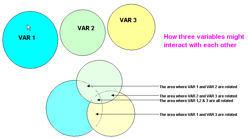
illustrated using a Venn diagram but do remember that the circles are intended
to represent balls (i.e. 3D) and not simply circles. Perhaps you might
consider them as 'flexible bubbles' that can change shape, merge and partially
cross through each other...

Our previous bivariate analysis methods would have yielded results in the 3 main overlaps (Pearson's Product Moment correlation would yield r-values) but we would not have been able to deal with the central 3-overlap situation. Yet it can be seen that if any one of those circles (variables) changed in size, then the context of the central 3-overlap would change also. It may be that the 'information' 'buried' in the central 3-overlap is what we really want to investigate and all the techniques so far discussed will only allow us to look at the three 2-overlap relationships.
It is not realistic to try to undertake these types of analysis without the use of a powerful computer software package.