abc
Level I STEP 8
Discriminant Analysis...."building a predictive model" |
However, the situation arises where we require a prediction / decision; not in clear quantitative terms but in terms of a qualitative judgment but still based upon sound mathematical principles.
In practical terms, this usually takes the form of a question; "we know we have categories but which category do we place each particular object into"? What are the parameters?
An essential prerequisite for Discriminant analysis therefore is that the groups are already defined (possibly with the aid of an ANOVA test) prior to analysis.
When we discussed Cluster analysis, we confined ourselves to clear distinctions with respect to the characteristics being recorded.
But...
|
What if the displayed characteristics (of the object) are unclear? What if this creates some indecision as to which group a particular object belongs? What if an object could conceivably belong to more than one group? |
Some terms of reference to allow us to discriminate between the a priori groups and a method of allocating new cases to the most appropriate group (with the minimum risk of making a mistake) are required. Again, it must be emphasised that only parametric data is presented for analysis.
As stated, for this type of analysis to work, the categories ( groups) must be defined a priori and the task is then to find the best functions / components (in canonical order) that best discriminate (i.e. maximise the distinctions) between the groups.
Suppose the RSPB decide to carry out a large national survey about the state
of the Barn Owl population in Britain. They can gather data concerning distribution,
absolute numbers, numbers of young, weight of birds, longevity etc. etc. The
crucial question however, may be; "which birds (or rather which groups
of birds) are most at risk"?
We could now invent two different groupings....'those at risk' and 'those not at risk'. Of course we might have to consider using more than just two groups. More importantly, it may be that we need to establish in advance the true mathematical nature of the difference between the groups; this might be achieved by carrying out an ANOVA test. There is little point in carrying out a Discriminant function analysis if the groups don't really exist but are simply wishful thinking or an artificial contrivance!!
After collecting all the numerical data we wish to place all the birds into one or other of the two categories. Such information could then be valuable in developing policies to help safeguard the more vulnerable populations of Barn Owls.
The concept of the analysis technique is to 'combine' those independent variables statistically selected (by the SPSS procedure) into one new single variable called the Discriminant function. Each case in the dataset earns a 'score'. These scores will be set in such a way as to discriminate to the maximum extent the differences present within the cases measured. We should find that there is the equivalent to a significant difference between the groups. A test statistic that SPSS will generate called Wilks' lambda will test the suitability of each independent variable for inclusion as part of the analysis and to assess the degree of discrimination that has been achieved.
If we are only considering two potential groups, it may be helpful to imagine two overlapping normal distributions, one for the 'not at risk' birds and one for the 'at risk' birds. Both curves would have their own mean and the task of the discriminant analysis procedure is to generate scores that place each case in one or other of the groups in such a way as to maximise the distance between those two means.
Within the procedure there are also techniques to help to discern those independent variables that make the greatest contribution to the process of prediction of the dependent variable.
We can use a stepwise procedure whereby each individual independent variable (often seen written as the Predictors) is inserted or removed from the analysis in turn. This allows the choice of which independent variables should go forward into the final steps of the analysis. The Wilks' lambda statistic is generated and the changes in its value (when a variable is left in or taken out) is recorded. The significance of this change is measured using an F-test. Only variables with an F-value greater than the critical value are allowed to proceed. SPSS will do all this for you.
So we have to go through a lengthy process of inserting and deleting and reinserting all the independent variables.
At the end of the analysis SPSS will produce a decision rule that will allow us to define mathematically which group any future individual (measured in the same way) is most likely to belong to.
We will also generate a '% score' that tells us how accurate we have been with our allocations of entities into their respective groups. There is little point in allocating an entity to a particular group if we are not satisfied that there is a reasonable chance of getting it right!!
The technique has applications in taxonomy where distinctions between subspecies may be very difficult to discern with the naked eye....
The Forestry Commission
are keen to explore the possibility of being able to identify the source of
felled trees simply by using a database of existing parameters such as height,
girth and cone length etc. To be able to rapidly identify which forests any
consignment of logged timber came from would help in the control and containment
of timber pests and diseases worldwide.
A pilot experiment was devised and began with sampling at three plantations in Scotland. Scots Pine trees (all of the same variety) were used. These trees manage to develop slightly differently depending upon many environmental factors such as soil type, drainage and exposure etc. Essentially however, they all look very similar to each other to the untrained eye.
5 biometric variables (the data must be parametric) were chosen and 20 trees selected at random from each of the three locations. You should understand that the 'Groups' are already known in that they are in fact the 3 plantations and we know which plantation each tree comes from. Thus 'Location' is the 'Grouping variable' here.
Discriminant analysis is going to eventually tell us how many trees conform to the 'signature' biometrics of their group and how many might more readily belong to one or other of the other two groups.
The variables that were considered easy to assess were :
1. Height (m)
2. Girth (m)
3. Cone length (cm)
4. Cone diameter (cm)
5. Canopy circumference (m)
Here is the dataset:
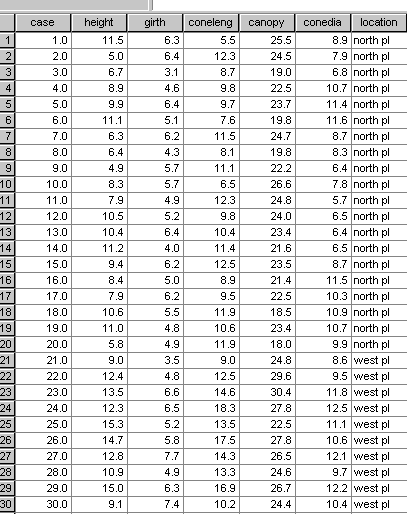
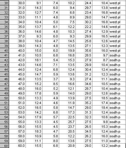
As always, we must first check the data for extreme values. We should remove them from the data set and allow SPSS to create means in their place. Any outliers present, we will leave in place...
3 x 20 trees in total:
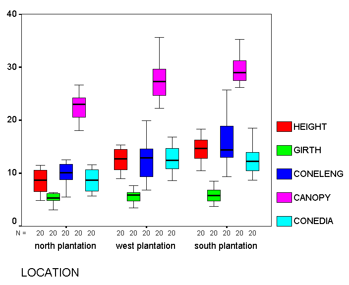
Essentially this will be satisfactory for analysis, there are no outliers and no extreme values.
Remember that each 'box' represents the results from 20 trees in just one plantation. If all the trees were from the same group, we would expect to see little variation between the groups. Look at the boxplots for 'height' for example; they look very different for each plantation. This may of course be due to environmental factors such as soil type (as already intimated) but the variation might be explained by suggesting that there is a differing proportion of taller members mixed with the shorter members in each plantation.
Q. Would it be fair to say that trees seem to grow taller in one particular plantation?
So the purpose of this Discriminant analysis will be to confirm and explore the groupings and then to predict the proportion of trees in each plantation that appear to belong to each group. It is very likely that the stepwise analysis that SPSS will perform will delete one or more of the factors measured as failing to be significant and we will be left with those variables that have contributed the maximum effect to the variability recorded. In practice, SPSS does things the other way round....all factors are discounted and then 'let back in' one by one.
Open SPSS and enter all the variables as shown above. Switch to Data view and enter your data.
Open 'Descriptive statistics', 'Explore'. Transfer 'Location' to the Factor box, 'Cases' to the label cases box and all the Dependent variables (predictors) to the Dependent list box. Click OK. This will generate individual boxplots for each variable.
Alternatively, for a more succinct output, go to 'Graphs', 'Boxplots', tick 'summary of separate variables'. Define: category axis: 'Location' and place all other predictors (other than 'cases') into 'Boxes represent'. Click OK. This will generate the boxplot shown above.
Open 'Analyse', 'Classify' and 'Discriminant'. Transfer 'Location' to the grouping variable box and define the range as 1 - 3 (i.e. Plantations 1, 2 and 3). Transfer all the other variables (other than cases) to the 'Independents' box. Click "use stepwise method".
Click 'Statistics' and also tick 'means'; 'Pooled within group matrices', click 'Continue'.
Click 'Method', 'Wilks' Lambda' and 'Display summary of steps'
Click 'Classify' and tick 'Summary table'
Click 'Continue' and OK
Be aware that the SPSS output for this analysis is extensive and will consist of at least 15 tables! Only the essential elements will be presented here......

Note that the matrix is a mirror image of itself aligned along the top right to bottom left axis.
Let us start by examining the various correlations. The values contributed by all 60 trees are taken into account at this stage. All correlations are quite weak, the strongest being between 'Height' and 'Cone length' (r = +.262) and the strongest negative correlation is between 'Cone length' and 'Cone diameter' (r = -.209).
A scattergraph illustrates the point....
Open 'Graphs', 'Scattergraph', 'Simple' and transfer the two variables as usual.
Double click to open as a chart object. Click 'Options' and 'Fit Line'
Click OK.
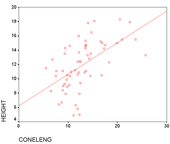
So far, we are not yet trying to distinguish between groups but simply examining all the possible relationships (and the strength thereof) that exist between any pair of predictors.
Output 6 indicates which variables have been entered into the analysis and which have been removed because they failed to comply with the Wilks' lambda criteria. The summary below shows that only three of the five variables qualify in the final analysis...
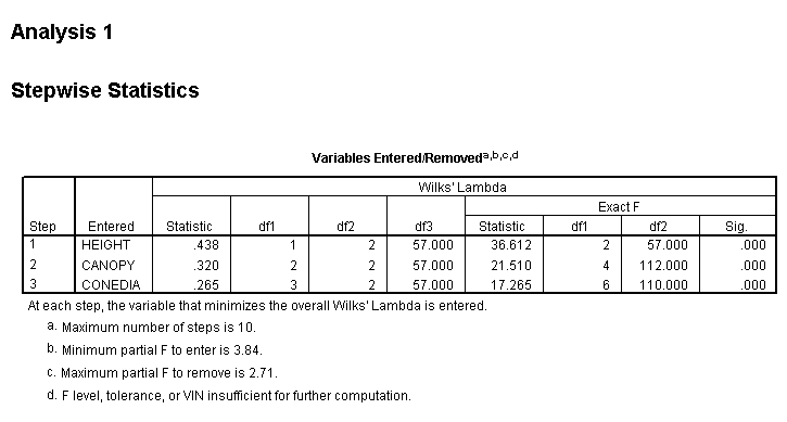
Note the minimum level for F required for entry is 3.84 and the maximum value prior to removal is 2.71....
The analysis is now explained in greater detail:
In step 1(second table below), you will notice that the variable with the highest 'F to enter' value is the one permitted to enter the continuing analysis. So initially HEIGHT enters with a value of 36.612.
In the next step CANOPY yields a value of 10.319 and is allowed to enter.
In the next step CONEDIA yields a value 5.662 and is allowed to enter.
In the next step NO VARIABLE yields a value of 3.84 or more and none are allowed to enter.
Notice how the 'F to remove' value changes as each new variable is allowed to enter. This is because it would then be necessary for any variable that yielded a revised F-value below 2.71 to be removed again!
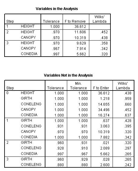
So after this third 'run' SPSS stops the analysis as there are no more variables that can enter.
Notice also that HEIGHT is the first variable to gain entry into the analysis because it achieved the highest F value. If we study the STEP 0 column you will see that it is the three variables with the highest F values that are eventually allowed to enter one at a time and in descending order.
Let us try to summarise what has happened so far with SPSS having run the analysis:
|
Initial
position
|
No
variables IN
|
|
After
first run
|
1
variable IN 4 variables still OUT
|
|
After
second run
|
2
variables IN 3 variables still OUT
|
|
After
third (and final) run
|
3 variables IN 2 variables still OUT
|
|
STOP |
We are now ready to examine the newly constructed Discriminant function(s)....
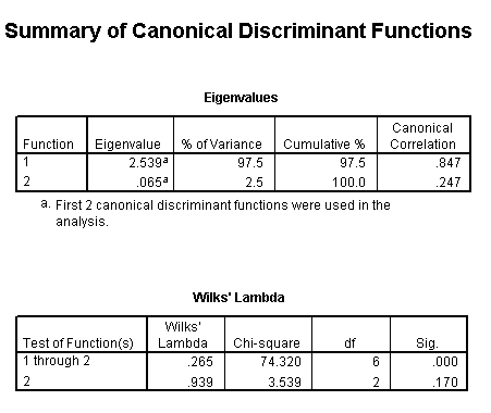
Two discriminant functions have been generated, the first accounting for 97.5% of the total variance recorded in the dataset and with P<0.05 and the second discriminant function accounting for the remaining 2.5 % of the total variance. Wilks' Lambda shows only the first discriminant function to be highly significant. The second discriminant function is not significant.
The next SPSS output examines the 'makeup' of the two discriminant functions that have been generated.
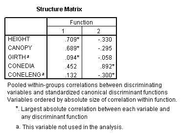
We can now see that the first function is contributed to positively by height and canopy and cone diameter.
The second (or lesser) function is contributed to positively by cone diameter and negatively by the height and canopy.
Thus we obtain the 'decision rule' for this particular dataset:
|
Discriminant function 1 is made up as follows: (.709 x height) + (.689 x canopy) + (.452 x cone diameter) Discriminant function 2 is made up as follows: (.892 x cone diameter) - (.330 x cone diameter) - (.295 x canopy) |
Prior to the analysis we would have had no other choice but to suppose that the distribution of groups within the three locations was evenly distributed just as SPSS indicates...
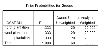
But the classification of "how many trees are in their most likely groupings" shows a different story...
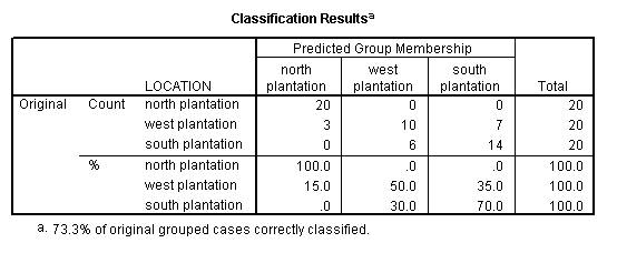
The 'predominant tree type' for the north plantation constitutes 100% of that sample.
The 'predominant tree type' for the west plantation constitutes 50% of that sample.
The 'predominant tree type' for the south plantation constitutes 70% of that sample.
We will see that there are 3 trees in the west plantation that have been predicted as (biometrically) belonging to the trees in the north plantation. The remaining 7 trees in that sample align more closely with those currently growing in the south plantation.
20 + 10 + 14 = 44 trees (out of 60) have been correctly classified (because we knew which group / plantation they were growing in) by Discriminant analysis and 44 / 60 = 73.3 % as indicated.
In other words, the output indicates that our overall success rate for being able to correctly predict the profile / 'signature' of the membership of a given group based upon the 3 measurements of: height, canopy circumference and cone diameter alone is 73.3%.
Illustrating that we have "maximised the divergence between the groups"
You will have noted from the Eigen values output that Discriminant function 1 accounts for 97.5% of the total variance present and so we will limit ourselves to exploring the information that just this one function can tell us. If we now complete the 'decision rule' calculations for 8 trees from each plantation (but only from those whose location was correctly predicted by the analysis), we will produce a new set of 'scores', one for each tree. This process is similar to solving an equation. The 'scores' produced are a distillation of all the data collected and then selected by the computer analysis. Each is a 'tag' or index that characterises that particular tree.
Remember: Discriminant function 1 is made up as follows:
(.709 x height) + (.689 x canopy) + (.452 x cone diameter)
E.g Tree 1:(North plantation and predicted to be in the North Plantation by Discriminant analysis output)...
So: (.709 x 11.5) + (.689 x 25.5) + (.452 x 8.9) = 8.15 + 17.57 + 4.02 = 29.74
'29.74' has no units and must only be regarded as the 'tag', index or 'marker' value for that particular tree but of course each tree will render it's own figure, so in this sense we have produced a 'new' variable and each case will have a value w.r.t. that new variable. We could perhaps label this new variable as 'Tree signature'.
Here is the data and the boxplot it yields...

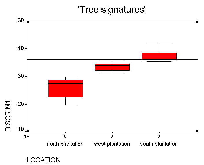
Because we have chosen to only work with the first discriminant function, we can only use a boxplot to illustrate the data. If we used 2 (or 3) discriminant functions, we could generate a 2D ( 3D) scattergraph and hopefully the points would form 2 (or 3) distinct 'clouds' of points. You can see that the analysis has maximised the variation present so as to make the maximum distinction between the three groups.
Another capability of Discriminant analysis naturally follow on from this point.....
Predicting Group membership (a tree from an unknown location)
This feature is may be considered of secondary importance but it is nevertheless a useful feature to understand.
Suppose that we wish to predict which grouping a particular tree is most likely to belong to, we can enter the values for the three eligible variables and by re-running the discriminant analysis, clicking 'save' and clicking 'predicted group membership', SPSS will utilise the values generated in the 'decision rule' to estimate which group the new tree is most likely to belong to.
SPSS will then insert it in the chart as shown in our added case (61) below.
The 'signature value' calculated from the 'decision rule' works out to be 36.04 for this tree and this line is marked on the Boxplot above. SPSS would place this value in the South plantation (and it does!!)....

This final output will also give the location that best 'fits' the biometrics of each tree measured. Look at cases 58 and 59 above, although certainly growing in the South plantation, their 'signature' is more closely aligned with those growing in the West plantation. Tree 60 seems to be in the correct plantation already!
So the Forestry Commission experiment has established that it would be possible to predict where a tree has come from simply by using a scale devised by measuring just three variables on existing trees. The accuracy of such predictions would be 73.3%.
As an extra facility, using SPSS, we could also plot the three selected original variables against each other on a 3D plot. This begins to show that there are 3 'groupings' present but that the points are confusing in that they appear to overlap each other to some extent.
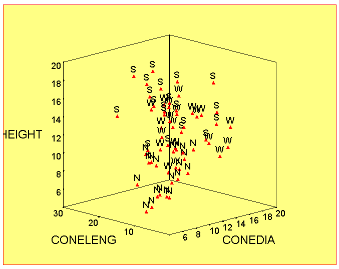
['S','N' and 'W' refer to the three plantations.]
This situation is improved upon (as already suggested), post analysis, by using the generated discriminant functions and the decision rule (instead of the original variables) to replot each tree either on a 2D or 3D plot to highlight and maximise the divergence between the 3 groups.
Q. Suggest ways in which the accuracy of the predictions might be improved.
But in a forest nearby....
An old forest of Fir trees in Scotland is known to consist of a number of subspecies; Pinus robusta, P. correcta and P.rotunda but this has never been verified. These subspecies are difficult to distinguish simply by eye and it usually requires some laboratory work.
Can we more readily identify these trees by measuring a number of variables such as tree height, girth etc.?
Again, we will be attempting to 'sort out' all the trees in our sample and we will try to discriminate between them so that they can be placed in their correct groups. For discriminant analysis, we must know in advance that groups do exist. If there is any doubt on this point then PCA must be used first.
33 trees were selected at random (from different parts of the forest) and accurately measured.
It was decided that 5 parametric variables should be examined:
1. Tree height
2. Tree girth
3. Bark thickness
4. Cone length
5. Cone diameter
Here is the dataset:
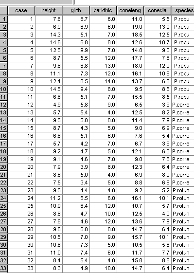
The grouping variable in this case is 'Species'.
Once again, we must explore the data looking for anomalies. Use the 'Analyse', 'Descriptives', 'Explore' functions in SPSS. Request Boxplots.
The output indicates that there are no anomalies to contend with....
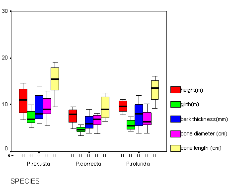
The results from the 3 subspecies look predictably consistent throughout (compare this with the boxplot in the earlier example) and for all 5 variables.
Q. Does this suggest that we might be wrong and that there is no evidence of subgroups ( distinct species) being present?.
There are no outliers so we can continue with the analysis..

We can see that there is a strong positive correlation between cone diameter and cone length (r =.637)
Q. What else does this output tell us ?
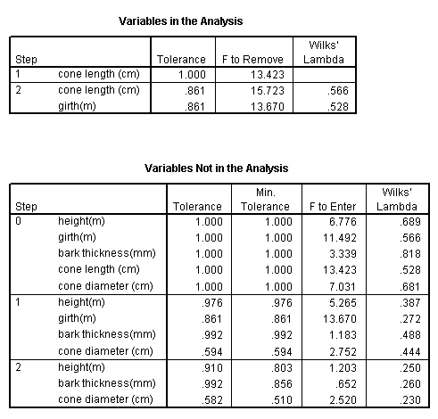
Task: Interpret the two outputs shown above.
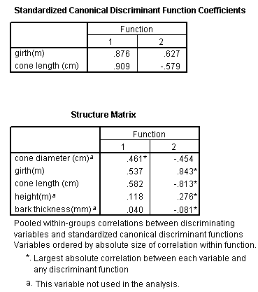
Task: Construct the two discriminant functions from the above outputs.
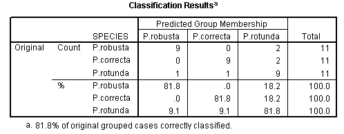
We have been able to correctly identify 9 out of 11 trees in each species, that is 27 / 33 = 81.8% of all trees evaluated. It is only necessary now to measure the girth and the cone length for us to classify another Pine tree in the plantation with approximately a 4:1 chance of being correct...
Task: use your derived 'decision rule' formula and the following data to identify the species of these two trees as far is practical....
|
GIRTH (m)
|
CONE LENGTH (cms)
|
|
|
case 34
|
6.8
|
7.3
|
|
case 35
|
9.5
|
11.1
|
SUMMARY
The three procedures (PCA, Cluster and Discriminant) all have one thing in common....they are all attempts to uncover hidden patterns or structure in complex datasets. They require no preconceived hypothesis but an open mind for their interpretation will help!!!
In STEP 7 (with PCA), we saw that it is possible to distill data down to it's 'essence', i.e. data reduction. Then, by generating some new 'composite variables', we might also determine if any natural 'clustering' into groups is indicated by the data.
We then saw how Cluster analysis is a concerted attempt to separate many entities into groups or clusters (if such groups really do exist) by quantifying their similarities / differences and even to quantify the 'distance apart' between all the individuals. Also, cluster analysis methods include some techniques that can be used with non-parametric data. These techniques, coupled with the use of Dendrograms are powerful ways to uncover relationships between related entities.
In STEP 8, we again show that it is possible to place objects into pre-proven (and therefore pre-existing) groups based upon their numerical profile and to go further by predicting the most likely group membership of a new individual.