 abc
abc
Level C STEP 7: Linked page
Pearson's Product Moment Correlation Coefficient |
We have seen that a correlation test can be performed using the Spearman test if one or both or the variables falls on the Ordinal scale.
Following on from that, if both variables reach the Interval or Ratio scale... and are Normally distributed we can use the more robust Pearson's test. The actual theory behind the test is different but the outcome is similar in that we eventually calculate r (the Pearson correlation) and the possible range is still -1 through zero to +1. Remember, as the r value approaches +1 or -1 so the association gets stronger and at zero there is no association between the variables at all or so it would seem...
Always bear in mind though that your experimental designs (or field observations) are rarely so pure that you can state with certainty that the variables you have chosen to measure have not been affected by some other non-recorded influence. Neither animals, people or environmental systems are ever that straightforward. Always be clear but cautious when drawing your conclusions.
One very important difference in this test is that we must use the actual values (and not resort to using ranks) e.g. weight Vs length or pH Vs number of organisms or rainfall Vs temperature etc. It is here that we can see that the PPMCC test is going to be more robust as there is no 'condensing' of the data and no arbitrary ranking.
Another difference is that our d.f will be (n - 2).
Remember once again to construct a scatter plot before commencing the analysis because it will give you a good early indication of what r is going to be and will reassure you that you have done the subsequent calculation correctly.
The manual procedure requires a rather lengthy table to be constructed because we need to calculate x, y, x squared, y squared, xy and sigma for each of these 5 columns as well as sigma x squared and sigma y squared!!
The
Null hypothesis is tested by comparing our PPMCC test
statistic (r) with a critical P-value from the tables.
As with Spearman's test, we have to reject the Null hypothesis if the test
statistic (r) falls outside of that +/- range indicated
by the critical value.
 We will start with a simple example: "Is there any correlation between
the hours of sunshine in Bournemouth and the amount of rainfall".
The Null hypothesis will be that there is no correlation between these two independent variables.
Ho: r = 0
The alternative hypothesis will state that there is a correlation between the two independent variables.
The test is two-tailed..why?
Readings were taken daily for 2 weeks (n = 14)...
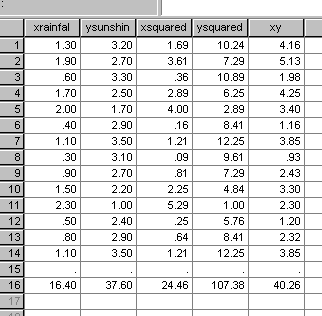
note that row 16 shows the sums (sigma) of each column
We have also calculated (Sigma x, 16.4) >>>squared = 268.96 and (Sigma y, 37.6)>>> squared = 1413.76.
So in total we need 7 mathematical values to do the calculation.
Do be very
clear that you appreciate the difference between  ...in the above example, the former would be 24.46 and the latter would be
16.4 squared = 268.96.
Next prepare the scatter graph either in Excel or in SPSS...
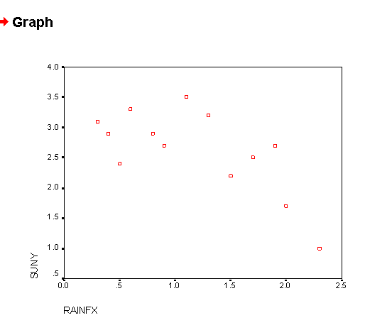
Q. What can you say about the relationship between x and y so far?
The formula to use looks daunting but once you have completed the table (as above) it is really quite straight forward. This is a clear example where the computer has the advantage over a manual system but it is still essential that you appreciate how and why a particular result is obtained before relying too heavily upon an SPSS output. This formula may look daunting but
 |
Here is the full maths workings to show that they are not that complex if you simplify in set stages...
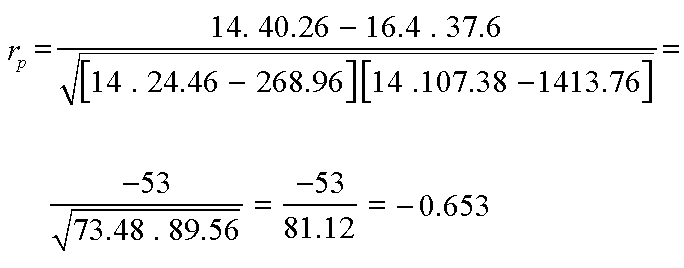
So r = -0.653
Check back to the scatter plot. Does this result seem to agree with the display?
So there seems to be quite a clear negative correlation but is the result significant? After all, our sample size is quite small and as we have often warned, do not be tempted to draw definitive conclusions where small sample sizes are concerned unless you have properly tested for significance.
Remember
what the confidence (P-value) is telling us in these cases.
We are only ever able to look at samples but it is really the whole
population that we are interested in so we are saying in effect "how
confident can we be that our result would accurately reflect the true situation
to be found in the whole population?".
P (0.05) (d.f = 12) = ± 0.576
Our test statistic is outside of this critical value and so we must reject the Null hypothesis and accept the alternative hypothesis viz: there is a significant correlation here.
In conclusion we can say that there is a definite negative correlation between the amount of sunshine and the amount of rainfall and that the result is significant at the 5% level.
In simple terms, the higher the rainfall, the less the sunshine! (Care! there may be other factors that can influence our weather so as always; be very careful about drawing rash conclusions from your research.)
P(0.01) = 0.708
Q. Does this change our conclusions at all?
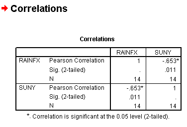
If you wish to check the calculation using SPSS, your output should look like this.
(The procedure is exactly the same as for the Spearman test except you tick the Pearson box instead).
Here is another example but in this case we have 3 variables (all clearly parametric ) to consider....
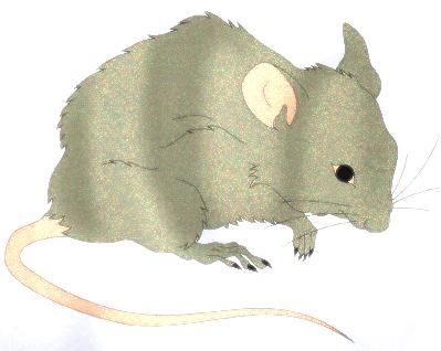 We
wish to investigate whether there is any association between body length,
tail length and body weight in 30 laboratory mice.
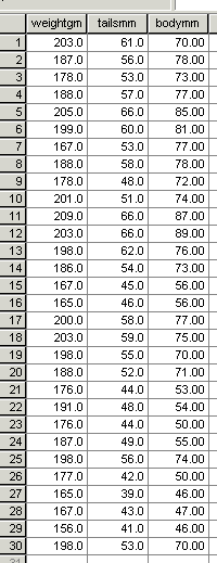
You will now be able to calculate three different Pearson correlations.
SPSS will generate a 'correlation matrix' if all 3 variables are carried over (in 'Bivariate data')....do not confuse this procedure with 'Multiple correlation'.
Comment upon the three rs values you have obtained.
Sometimes, the distiction between parametric and non-parametric variables can be blurred. pH is one such instance because it is already a log value. In such cases, it can be useful to run both a Pearson's and a Spearman's test.
Another SPSS data set to work through....
 The recolonisation of landfill sites by pioneer plant species is to be investigated.
Generally such soils will be quite acid. It is thought that by optimising the soil pH (with Lime) that a greater and more rapid colonisation and improvement in biodiversity can be achieved. The Environment Agency have commissioned you to investigate 20 completed landfill sites.
You must record the number of plant species found at each site along with the overall soil pH of that site. Remember to produce a plot first..
|
Site |
Number of Species found (x) |
pH (y) |
x squared |
y squared |
xy |
|
A |
35 |
4.2 |
|||
|
B |
36 |
3.7 |
|||
|
C |
41 |
4.4 |
|||
|
D |
28 |
2.9 |
|||
|
E |
40 |
5.7 |
|||
|
F |
45 |
4.8 |
|||
|
G |
25 |
3.3 |
|||
|
I |
48 |
6.7 |
|||
|
J |
36 |
4.9 |
|||
|
K |
22 |
2.8 |
|||
|
L |
30 |
5.7 |
|||
|
M |
39 |
5.8 |
|||
|
N |
44 |
6.6 |
|||
|
P |
31 |
3.5 |
|||
|
Q |
32 |
4.0 |
|||
|
R |
26 |
2.8 |
|||
|
S |
28 |
5.7 |
|||
|
T |
41 |
6.6 |
|||
|
U |
44 |
6.9 |
|||
|
V |
34 |
3.7 |
TASK: Using SPSS, Calculate the Pearson & Spearman r values and P-values and write your conclusions in the form of a brief report for the Environment Agency.
Q. What recommendations (based upon your findings) would you make about future research into the subject?
This concludes Level C.... Well Done!