 abc
abc
 abc
abc
It would be wise to make sure that you comfortable with the outcome of the Question / Perception material for level C before proceeding.
Level C was designed to cover all the essential prerequisite topics that are necessary in order to manipulate, describe and begin the process of making inferences from all types of collected data.
In Level I, it will become increasingly apparent that the capabilities of inferential statistics run deep. As a consequence, the maths becomes more involved and so there is a much greater reliance placed upon the use of SPSS. This program should be regarded as an 'Industry standard' for this type of work.
We begin by reconsidering the nature of data, how it can be handled and how it can so easily be mishandled. We reinforce the essential need to ensure that all the data you try to Analyse is in the correct format and is reliable. If you commence with dubious data, there are no tests at all that will rectify that situation. There is no such thing as perfect data but you have a duty to ensure that your material is as accurate as is practicable.
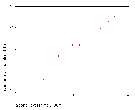
At the end of Level C we discussed how the use of Correlation allowed us to determine if a relationship existed (and its strength) between two variables. The companion technique of Regression sets out to produce a model of that relationship with a view to being able to 'predict' values for one variable just by using known values for the other. The use of scattergraphs is central to this process. The idea of 'the line of best fit' is explained and the process of interpolation is introduced...

There now follow 4 pages (STEPS 3, 4, 4 link and 5) devoted completely to the analysis of variance. This is potentially a vast topic.
You will recall that t-tests are used to test for differences between the means of two samples. Analysis of variance is an extension to this concept in that it allows us to test for significant differences between 3 or more sample means. Again, the main point to grasp will be the issue of whether the observed differences between the sample means has occurred by chance (through sampling fluctuations for example) or whether the differences are so large that it is unlikely that they occurred by chance. There are at least 5 sub-groups of ANOVA and although it is not intended that we look at all versions, we will look at one-factor, two-factor, repeated measure and the ANalysis of COVAriance.
Not only will these techniques be useful to the researcher but they will also give you practice and experience in manipulating large datasets.
Next we look at Principal Components analysis which is a multivariate technique that allows us to examine a matrix of correlation coefficients (for three or more variables) all at the same time!! It is a difficult concept to grasp but the idea is that the the number of variables 'in play' is distilled in such a way as not to loose any of the inherent information contained within the original dataset. The term often employed here is 'dimension reduction'. Furthermore, those variables most responsible for the bulk of the variance displayed are highlighted and their relative importance is exposed. We will then deduce the multi-dimensional nature of the data and look for evidence of 'clustering' within the data.
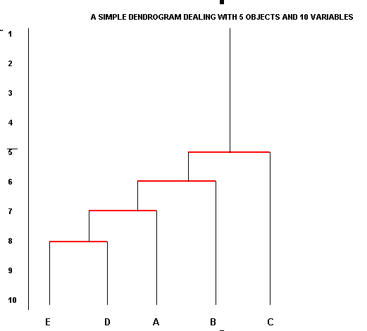
Another type of data reduction can be achieved by using Cluster analysis. This is derived from the ancient idea of using specific (usually visible) characteristics to 'pigeonhole' objects into their 'natural groups'. Cluster analysis deliberately sets out to highlight any natural groupings that may exist. Two complementary Non-Parametric techniques are explained here; one just looks at similarities between objects and the other looks at similarities and differences. The use of Dendrograms is explained.....

Discriminant analysis takes the issue of "which group does an object belong to" one stage further. Groups have to be are assumed a priori in this analysis. As with PCA, the key idea to grasp is that each variable (that remains represented as the analysis progresses) becomes distilled into 'components' and is finally represented as a dimension in space. By extracting those new 'components' (from the variables) that contribute the most to the observed variation, it is possible to measure and maximise the 'distance' between all the groups. By then gauging those same parameters for each object it is possible to 'lock' each object onto the most appropriate grouping. We can produce 2D (and sometimes 3D) plots which will show the results of this manipulation as 'clouds' of data points.
Finally we take a brief journey into Spatial statistics and look at Nearest Neighbour analysis.
This is a technique much favoured by Ecologists and Geographers to describe plant distribution patterns and to compare an observed distribution of points (such as churches, wells or petrol stations etc) with theoretical random ( or otherwise) patterns. The method is based upon measuring a physical distance between each point and its' nearest neighbour and calculating the mean of all those distances with an expected mean if the pattern were completely randomly placed.
There are some concluding paragraphs that discuss two other spatial techniques that you may find useful; Point pattern analysis and Trend surface analysis.