abc
The paired t-test(a note about Standard error)(an explanation of 'degrees of freedom') |
This is the point in the package where we embark upon inferential testing in the truest sense.
We want to quantify the difference between two samples.The essential aim of this test is to assess the significance of any differences between the two sets of samples. Once we begin to think in terms of more than two sets, then t-tests are not sufficient unless a series of comparisons... A - B, A - C, B - C etc is contemplated.
The test is characterised by looking at the way the arithmetic means of two related sample sets behave. The greater the difference between the two means, the more likely it is that there is a real difference between the two sets.
Note however, that if the variability in the two sets of scores is great ( or the degree of overlap is great) then this will reduce the likelihood of a real difference existing.
So we need a test that can cope with these two interlinked factors.
't' is always an index and will be the 'test statistic' we are aiming for... it reflects the difference between the two means (of the two sample sets) and the standard error (S.E.) of that difference. We are really calculating how many times greater than the S.E. (of the difference) the difference between the means really is!!
Remember that the S.E. (of a mean) is simply the standard deviation of a set of arithmetic means from n samples. It is a measure of the average dispersion of the sample means about the population mean.
The paired 't'-test is a parametric test so we must use data that is on the Interval or Ratio scale.
It is very
common in many environmental investigations to want to compare "how things
were with how they are today". Once again we are a)
making comparisons (often over time) and
b)
looking to discover if things have got better or worse (which direction / 2-tailed).
Good scientific procedures will invariably try to eliminate as many variables as is practicable so that we are sure that when we make a comparison we are always comparing 'like with like'.
Paired data simply means that 'pairs' of results are to be compared. It may be a river (for pollution levels at two different locations) or a nesting site compared over two years (for breeding rates) or a power station over a winter and a summer (for sulphur dioxide emissions). The important point is that the two sets must be inherently related to each other. We will deal with the alternative case where the two data sets operate independently of each other on the next linked page>>>the unmatched t-test.
We need to more fully explain two terms before we can proceed....
S.E. (related to a mean) is simply a modified form of
the standard deviation of a set of arithmetic means from n samples. It
is a measure of the average dispersion of the sample means about the population
mean. Imagine that we wanted to measure the weight of lobsters caught in one
month.
We might decide to weigh them in batches of 5 and so each 5 will give us a mean weight for that batch. Understandably, if we repeat the process on different nights we are going to get a slightly different value for the mean of each sample of 5. However, the more we repeat the sampling the nearer the overall mean is going to approach the true mean catch weight for that population of lobsters in that month. So now, instead of calculating the standard deviation for each sample, we can calculate the S.D. for all the means that we have calculated and this is the Standard Error. The higher the number of samples, the more the various sample means approximate to the true mean and so the smaller the S.E. becomes.
If we know the means of the samples and the S.E, we can calculate 't':
So:
|
t = |
difference between the means |
|
S.E. of the difference in the means |
One definition is "The number of values (pieces of data) in a data set that are free to vary".
We use d.f. of the sample (n) (as opposed to taking the full population (N)) because we need to take account of the number of independent values we have extracted or sampled from that population. By calculating any statistic (such as the mean) we inevitably loose an independent estimate of the scatter....
Suppose we weigh 4 Oysters (gms):
|
80 |
160 |
|
140 |
180 |
The mean is 140gms
Now suppose we randomly pick out 3 oysters: 80, 140 and 160. The final sample has to be 180 in order that the mean should be 140gms. In other words, that last sample is not free to vary.
After calculating the mean from 4 independent data points; only three will remain independent.
So: d.f. = 4 - 1 = 3
Note that
where we are required to use (n - 1) that is; (population - 1 sample) the effect
is going to be much greater where n is small. If n = 10 then (n - 1) will make
a large difference but if n were 100, then
(n - 1) will make a very small difference. In fact, as n gets larger then (n
- 1) will approach n anyway!.
Hence the general philosophy in all statistics work; that you must make sure that your sample size is sufficiently large for your chosen tests to work properly. If you are faced with a very small dataset, do check carefully which tests you can legitimately use.
Note: Nonparametric tests do not use absolute values but use ranks, positions etc and so n is used (where required) with no adjustments.
You will also note that on your scientific calculators, that the standard deviation of a sample is labelled as s.d(n - 1) and that of the complete population is labelled as s.d.(n)
Let us consider a busy river estuary that became heavily polluted in the 1960's
with industrial effluent. Campaigners managed to convince the Local Authorities
that a 5 year 'clean up' campaign was urgently required. Environmental scientists
from the local University were asked to monitor the progress. They decided that
the number of benthic crustacean species present was a representative measure
of the changes in biodiversity in the estuary. The biodiversity is just one
possible benchmark that might be used to gauge the 'health' of the estuary.
Mud samples were collected from 8 locations (n = 8) within the estuary before the 'clean up' began and again (from exactly the same locations: hence the point about 'paired' samples) 2 years into the project.
Here are the results... (do not concern yourself with the two right-hand columns for the moment)
|
Location
|
No
of species recorded(after 2 years)
|
No
of species recorded (prior to commencement)
|
difference
(d)
|
each difference (d) squared |
|
for SPSS>>>
|
'AFTCLEAN'
|
'BEFCLEAN'
|
||
|
1
|
13
|
10
|
3
|
9
|
|
2
|
13
|
9
|
4
|
16
|
|
3
|
11
|
9
|
2
|
4
|
|
4
|
10
|
5
|
5
|
25
|
|
5
|
14
|
9
|
5
|
25
|
|
6
|
12
|
8
|
4
|
16
|
|
7
|
6
|
2
|
4
|
16
|
|
8
|
12
|
7
|
5
|
25
|
|
SUM
(Sigma)>>>>>>>>
|
32
|
136
|
Make sure that you appreciate that the data in columns 2 & 3 are paired and must not be separated from each other.
1) The Null Hypothesis: (be very precise) "There is no significant difference between the mean number of Crustacean species found before remedial 'clean up' began when compared with the numbers found to be present two years later".
The Alternative Hypothesis says that "there is a significant difference between the numbers of Crustacean species found before remedial 'clean up' began and the numbers found to be present two years later".
In mathematical terms we express this as:

2) We need a two-tailed test because we want to know if the results are simply different from before commencement. The numbers of species might have gone up or down.
3) Carry out the test: (Manually and then repeated using SPSS) always still assuming that the Null Hypothesis is true:
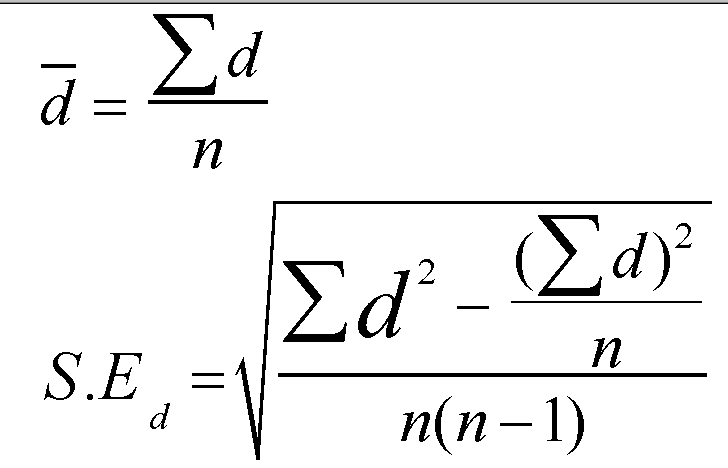
Firstly sum all the differences(=32), then calculate the mean difference (d bar) from:
d bar = sigma d divided by n
= 32 / 8 = 4
So this is the mean of all the differences generated by each pair of values.
Secondly, we need to calculate the standard error, both formulae are shown below:

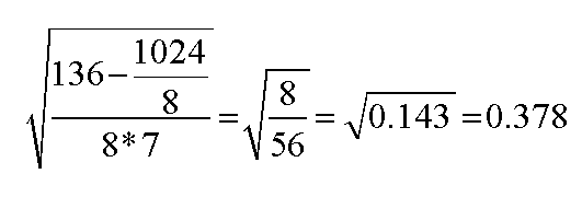
In the case of Crustacean species example, the formula for calculating the S.E. translates to:

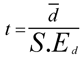
The third task is to calculate the test statistic (t): this is simply d bar divided by the S.E:

So: 4 / 0.378 = 10.582
Note that it is positive, as this is a two-tailed test the sign will tell us which direction the difference is in
4) Compare our test statistic with the critical value from the value for 't' tables in a textbook
The degrees of freedom for a sample is always (n - 1) and so in this case it is 7
Read off the figure for P(0.05) (df = 7) and it says 2.365 This then is the critical value for 't'
5) Our test result has exceeded this value and so the results are significant; we can reject the Null Hypothesis and accept the Alternative.
But going back to the table and reading off the value for P (0.01) (df =7) we see a figure of 3.499.
Q. What effect does this more stringent P value do to our Null Hypothesis?
6) Stating our conclusion
" There are significantly more crustacean species present after two years of remedial work than were present prior to commencement". (t =10.58, df = 7, P < 0.05).
Q. How would you write the appropriate hypothesis given P(0.01)?
Now we will rework the same example but using SPSS...
Open SPSS
Click 'enter data'
Open variable view
name the variables as: AFTCLEAN and BEFCLEAN
Open data view
Enter the data
Go to Analyse > Compare means > Paired sample T-tests
Highlight and transfer both variables to right hand box
Click 'Options', check that P is set at at 0.05 (95%) note that you can set other levels if so desired
Click OK
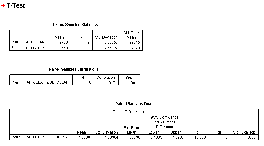
The output should look like this:
The first table tabulates the statistics for each variable. The second table indicates the correlation coefficient as .917.This is a topic we will cover in step 7. The final table in the output shows us the 't' value (10.583) and the P value.

Note that the Sig (2-tailed) value is shown to be highly significant by the .000 value shown. You may find that this notation is confusing but when using SPSS you must learn to recognise this format as part of the programme notation.